Visualizing adversarial examples with caricatures

Summary

Caricatures are a way to visualize an exaggerated version of what a layer within a neural network “sees”. They can be used as a way to visualize how each layer “reacts” to adversarial examples.

Two important terms: “adversarial examples” and “caricatures”

1. Adversarial examples

In simple words, an adversarial example is an image which has been engineered to “fool” a neural network, while being visually indifferent from that of a natural image to the human eyes.

The simplest way to do this is to use the FGSM algorithm: which is basically “training” the image to maximize or minimize the activations of a certain class within the neural network.

Adversarial examples are proof that even though deep neural nets seem non linear, their linear nature at a smaller scale (y = wx + b) can be very easily exploited.

To know more about adversarial examples, you might out to check this out.

2. Caricatures

Ever seen cartoons of famous people drawn in a way to exaggerate their features (eyes, nose, etc) ? They’re called caricatures.

They’re an exaggerated version of what one sees.

How are caricatures relevant here ?

Imagine a 2 layer neural net with 2 layers P and Q

So the model looks like:

class model(nn.Module):
    def __init__(self, p, q):
        self.P = p  ## p and q are imaginary layers
        self.Q = q

    def forward(self, x):
        '''
        x_p is an encoded version of x
        '''
        x_p = self.P.forward(x)
        x_q = self.Q.forward(x_p)

        return x_q

So now let us ask this question:

Is there a way to reconstruct the input image given a layer encoding x_p ?

The answer is yes, let me explain:

First let us feed an input image X_original into the model, and save the encoded version as X_original_encoded.

Now let us prepare a trainable image parameter and call it X_trainable.

After feeding X_trainable into the model, we get an encoded version of it called: X_trainable_encoded

Since X_trainable and X_original are not the same,X_original_encoded and X_trainable_encoded are also not the same.

Which means we can simply make them more similar by minimizing the loss between X_trainable_encoded and X_original_encoded.

So which loss function should be used ? ?

Initially I went for the MSELoss, but that did not provide much insight about the layer itself.

Then after some very interesting discussion with Ludwig from Distill Slack, I went for cosine similarity.

What on earth is cosine similarity now ?

Imagine you’re looking up at the sky during a solar eclipse.

you – moon — sun

How far is the moon from the sun ? very far

Therefore, the MSE loss between the position of the sun and the moon is very high. But how far do they look to the humans on earth ? very close, sometimes even on top of each other

Hence, the cosine similarity between their positions (with respect to earth as the origin) is high i.e 1.

Given 2 points, cosine similarity is calculated as the cosine of the angle between them w.r.t the origin.

If the angle between 2 points is high, then the similarity is low: cos(59) = 0.559

If the angle between 2 points is low, their similarity is high: cos(10) = 0.9848

I really don’t like to use fancy mathematical terms to explain things, so if you’re that kind of a person I’ll link you to this article.

That was quite an astronomical tangent, now let’s get back to caricatures

So our objective was to maximize the cosine similarity between X_trainable_encoded and X_original_encoded in an iterative manner.

This is how it looks like:

dreamy_boi = torch_dreams.dreamer(model)  ## wrapper over a pytorch model

for i in range(iters):
    
    X_trainable_encoded = dreamy_boi.get_snapshot(
        input_tensor = X_trainable, 
        layers = [model.P]
    )[0]  ##[0] because it returns a list

    loss = -(cosine_similarity(X_trainable_encoded, X_original_encoded))

    loss.backward() ## calculate gradients 
    X_trainable.optimizer.step()  ## update values
    

Notice the minus sign in the loss, that’s because we’re minimizing the loss i.e maximizing cosine similarity.

There’s one more problem left now, caricatures are supposed to “exaggerate” an image right ?

Cosine similarity looks like:

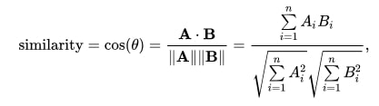
Now in order to “exaggerate”, we can optimize both the cosine similarity and the dot product.

This is how the usual loss function looks like:

loss = -(cosine_similarity(X_trainable_encoded, X_original_encoded))

And this is how the new “exaggerated” objective looks like:

exaggerated_loss =  -(cosine_similarity(X_trainable_encoded, X_original_encoded)*(X_trainable_encoded* X_original_encoded)**power_factor)

Note that V is the encoded version of the trainable image and U is the encoded version of the original image. Notice how in the 2nd version, V tends to move further away from the origin, that’s where the “exaggeration” is.

I skipped the weird section above, just tell me what did you mean by caricatures here

Caricatures here are an exaggerated version of what a layer of the model “sees”. You can consider them as a way to see a more extreme version of what the model saw in an input image.

Now back to adversarial examples

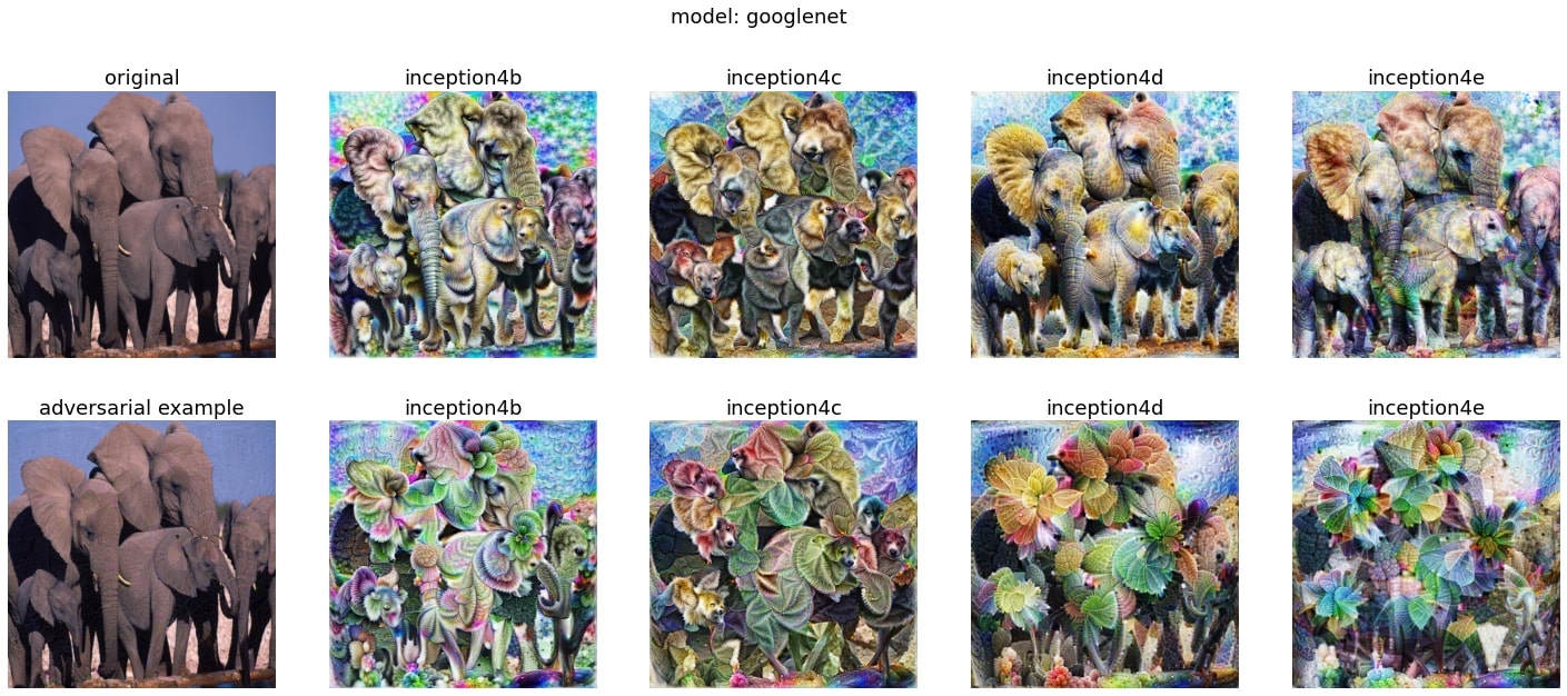
Let’s see what happens when we feed an adversarial image of an elephant which is meant to be misclassified as a potted plant.

Interesting to see how the layers “see” leaves instead of elephants to a higher extent in some layers than in others. This now raises the question of trying to find ways to look for “culprit layers” within the model which are “guilty”.

I just wrote this blog post as a way to document my findings while doing these experiments. If you do feel like discussing these ideas further with me, just drop an email: mayukhmainak2000@gmail.com