What does the paper try to prove ?
The use of transformers for vision has remained quite limited so far. We did see some weird mixtures of convolutional layers and attention, but it turns out that a pure transformer can also perform very well on image classification tasks.
The problem with conv layers
Conv layers are really good at detecting textures in images, but they’re not at all good at detecting large visual features (this is because of the fact that conv filters are just these tiny sliding windows).
Each conv filter has a limited receptive field, which grows as we go deeper into the layers. But transformers are able to attend to “everywhere on the image” within a single layer.
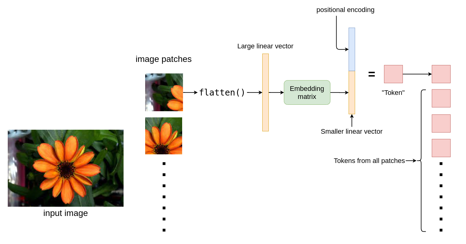
How do we “tokenize” images ?
“Let’s not do local attention over pixels, but global attention over image patches!"
This is how they did it:
- Chop down the image into 16x16 patches
- Flatten the patches
- Produce lower dimensional linear embeddings from flattened patches.
- “Add in/concat” positional embeddings.
And now we have our sequence of “tokens” which we can feed into the model :)
Hold up, what are positional embeddings ?
In simple words, they’re “vectors” which tells the transformer where every patch was in an image. These positional embeddings are learnable.

Given above is a a brief visual summary of how each image patch is tokenized.
What information does each “token” hold ?

“Enter” the transformer
Now that we have our “tokens”, the next step is to feed them into the transformer. Let’s first take a look at the original diagram which shows the insides of the transformer:

In order to better understand how each of those small boxes work, you should read this other post I wrote.
At this point I’ll assume that you already have a basic understanding of stuff like Layer normalization, multi head attention, residual skip connections.
The encoder architecture used here is the same as the one we know from the original paper.
There is no decoder, Just an extra linear layer for the final classification called MLP head.