First off, this is by no means an official guide/tutorial. If you’re stalking me, then this post wont be super useful. If you’re here by accident, then all that I can say is that life works in mysterious ways.
I’ll try my best to explain to myself and to you, the reader how Andrej Karpathy‘s minGPT works. All the source code you see here is taken (and maybe slightly modified) from the minGPT repo.
1. Building a dataset
import math
from torch.utils.data import Dataset

class CharDataset(Dataset):

    def __init__(self, data, block_size):
        chars = sorted(list(set(data)))
        data_size, vocab_size = len(data), len(chars)
        print('data has %d characters, %d unique.' % (data_size, vocab_size))

        self.stoi = { ch:i for i,ch in enumerate(chars) }
        self.itos = { i:ch for i,ch in enumerate(chars) }
        self.block_size = block_size
        self.vocab_size = vocab_size
        self.data = data

    def __len__(self):
        return len(self.data) - self.block_size

    def __getitem__(self, idx):
        # grab a chunk of (block_size + 1) characters from the data
        chunk = self.data[idx:idx + self.block_size + 1]
        # encode every character to an integer
        dix = [self.stoi[s] for s in chunk]

        x = torch.tensor(dix[:-1], dtype=torch.long)
        y = torch.tensor(dix[1:], dtype=torch.long)
        return x, y
So what’s going on inside __init__ ?
First, lets look at the arguments.
data: a long, long string which contains all of the training data. In this case it would be something short like that of a poem.block_size: number of characters to be included in the input/label. One can also think of it as the spatial extent of the model for its context.
And now the attributes:
self.stoi: weird name, which actually means “strtoint”self.itos: weird name, which actually means “inttostr”self.vocab_sizeis the total number of unique characters found within the training data.
if you print self.stoi, it looks like:
{'\n': 0,
 ' ': 1,
 "'": 2,
 '(': 3,
 ')': 4,
 ### its a lot longer IRL, I clipped it out :)
}
self.itos is basically the same thing but flipped around:
{0: '\n',
 1: ' ',
 2: "'",
 3: '(',
 4: ')',
 ### its a lot longer IRL, I clipped it out :)
}
In a nutshell, they’re just a way to map all of the unique characters in the dataset to certain integers.
Now let’s build a dataset:
block_size = 10 ## 10 is not a good number for training, but is good for intuition
text = open('input.txt', 'r').read()
train_dataset = CharDataset(text, block_size)
Let’s look at a single training sample:
x, y = train_dataset.__getitem__(0)
print('x: ', x)
print('y: ', y)
the output would be something like:
x:  tensor([10, 28,  1, 17, 18, 16, 17,  1, 27, 14])
y:  tensor([28,  1, 17, 18, 16, 17,  1, 27, 14, 10])
here, each number in x and y points to a certain character in the training dataset. Let’s see what x and y actually are:
def ints_to_readable(train_dataset, x):
    x_readable = [train_dataset.itos[i.item()] for i in x]
    return(''.join(x_readable))

print('x: ', ints_to_readable(train_dataset, x))
print('y: ', ints_to_readable(train_dataset, y))
output:
x:  at high se
y:  t high sea
That’s all for the dataset! before we move on to the model, here’s another interesting point mentioned in the original notebook:
So for example if block_size is 4, then we could e.g. sample a chunk of text “hello”, the integers in x will correspond to “hell” and in y will be “ello”. This will then actually “multitask” 4 separate examples at the same time in the language model:
- given just “h”, please predict “e” as next
- given “he” please predict “l” next
- given “hel” predict “l” next
- given “hell” predict “o” next
2. The model
The next step would now be to look at the model’s basic architecture, which depends mainly on the following factors:
- Vocabulary size of the dataset
- Block size of the dataset.
- Number of layers
- Number of attention heads
- Size of the embedding vector
The first 2 factors are already known from the training dataset. So let us look at the last 3 factors:
- Number of layers (
num_layers): The number of standard repeated layers to be used in the model. Higher -> deeper model. - Number of attention heads (
n_head): Check out this section I wrote in another blog post - Size of the embedding vector (
n_embd): It can be thought of as a lookup table which takes in a bunch of integers as input and returns corresponding “vectors”.
Wait, what are embeddings ?
They’re “learnable look-up tables”, which can be constructed with torch.nn.embedding:
import torch.nn as nn

embedding = nn.Embedding(3, 4)
print('embedding values: \n', embedding.weight.data)

print(f'embedding([0]): ', embedding(torch.tensor([0])).detach())
print(f'embedding([1,2]): ', embedding(torch.tensor([1,2])).detach())
would print something like:
embedding values:
 tensor([[ 1.5205, -2.2728, -0.0874,  0.4219],
        [-1.3103,  0.3491, -0.0410,  1.1601],
        [ 0.7829,  0.2559, -1.7153,  0.1395]])
embedding([0]):  tensor([[ 1.5205, -2.2728, -0.0874,  0.4219]])
embedding([1,2]):  tensor([[-1.3103,  0.3491, -0.0410,  1.1601], [ 0.7829,  0.2559, -1.7153,  0.1395]])
Also, what is layer normalization ?
Would recommend you to check out this section I wrote in another blog post.
Components
Self attention:
I’ve already explained how self attention works in another blog post, highly recommended that you check it out.
The difference here (CasualSelfAttention) is that it is has multiple heads, with an extra linear layer in the end.
The transformer block:
class Block(nn.Module):
    """ an unassuming Transformer block """

    def __init__(self, config):
        super().__init__()
        self.ln1 = nn.LayerNorm(config.n_embd)
        self.ln2 = nn.LayerNorm(config.n_embd)
        self.attn = CausalSelfAttention(config)
        self.mlp = nn.Sequential(
            nn.Linear(config.n_embd, 4 * config.n_embd),
            nn.GELU(),
            nn.Linear(4 * config.n_embd, config.n_embd),
            nn.Dropout(config.resid_pdrop),
        )

    def forward(self, x):
        x = x + self.attn(self.ln1(x))
        x = x + self.mlp(self.ln2(x))
        return x
Let’s first look at the GeLU actvation function.
import torch
import numpy as np

def gelu(x):
    cdf = 0.5 * (1.0 + torch.erf(x / np.sqrt(2.0)))
    return x * cdf
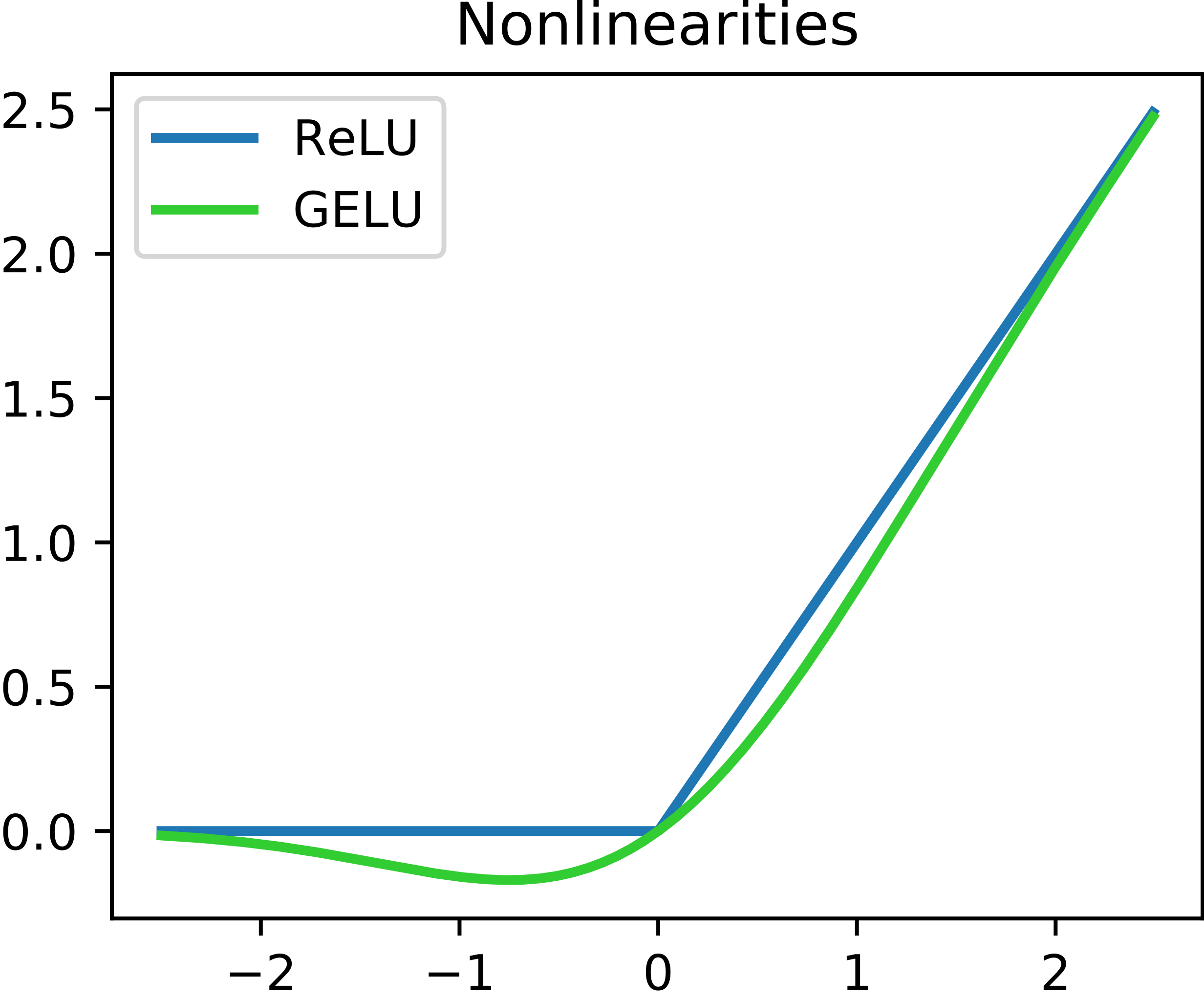
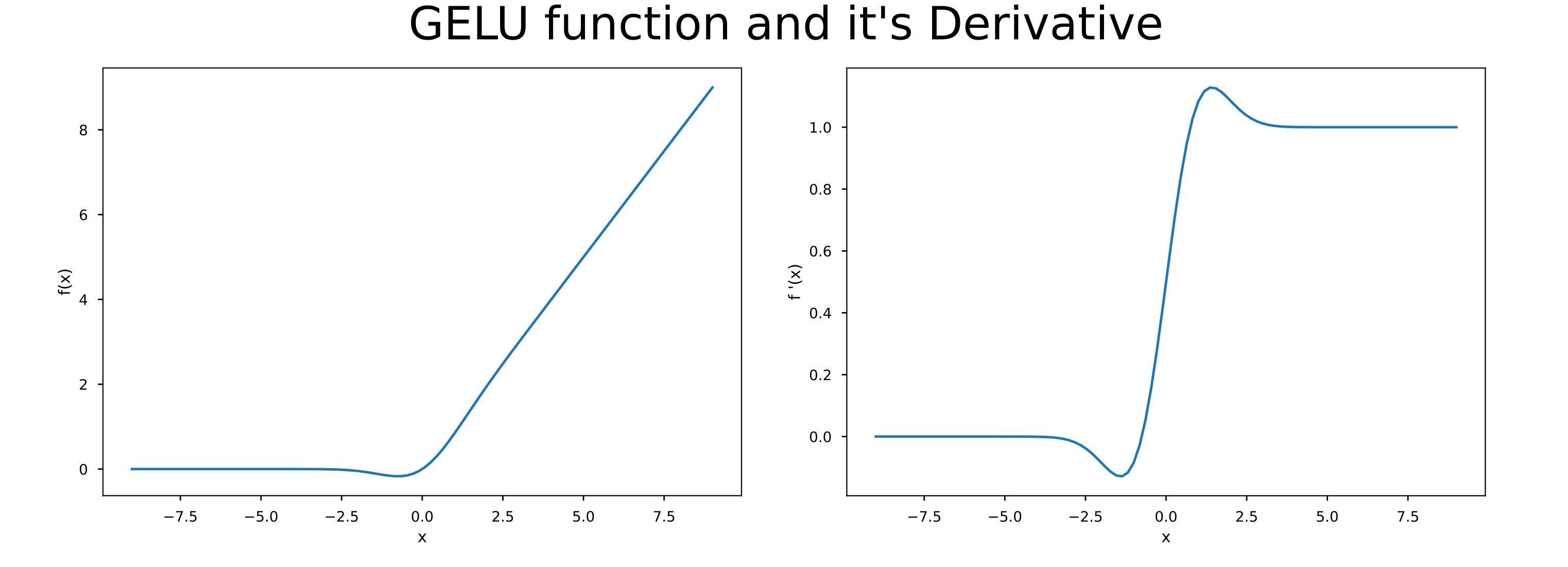
It should be visible from the image above how GeLU is different from ReLU. But the real interesting difference lie in their derivatives
The image shown above is taken from this blog post which is a great resource if you want to know more about GeLU.
3. Training
Abstraction
First of, let us see what the model actually does from an input-output perspective:
Given a sequence of characters, we first convert them to an embedding (a bunch of integers). For our example, we are assuming that the block size is 4. hence the length of the input along dim 0 is 4.
## ['p', 'y', 't', 'h', 'o']
x = [2, 6, 7, 8, 4]
Given the input sequence as shown above, the model has to predict the next “step” of the sequence. Something like:
y = model(x)
y ## ['y', 't', 'h', 'o', 'n']
>>> [6, 7, 8, 4, 3]
In reality, the output is of shape: [Block size, Vocabulary size]. So if the vocab size was 9, then the ideal output [6, 7, 8, 4, 3] is actually:
## shape: (4, 9) i.e (Block size, Vocabulary size)
[
    [0, 0, 0, 0, 0, 0, 1, 0, 0], # 6
    [0, 0, 0, 0, 0, 0, 0, 1, 0], # 7
    [0, 0, 0, 0, 0, 0, 0, 0, 1], # 8
    [0, 0, 0, 0, 1, 0, 0, 0, 0]  # 4
    [0, 0, 0, 1, 0, 0, 0, 0, 0]  # 3
]
Then if we run argmax over this output, we get [6, 7, 8, 4, 3].
Loss
The nature of the outputs of the model points to the fact that we’re “classifying” the next sequence of words from an input sequence.
For classification problems, we use the cross entropy loss. This blog post is a great resource in case you’re not familiar with it.
The special thing to notice here is that this is not your regular classification problem. Instead it is actually n
classfication problems stacked up (where n = block size).
Hence the loss function looks like:
import torch.nn.functional as F

'''
block_size: 10
vocab_size: 33
'''
x = torch.tensor([1,2,3,4,5,6,7,8,9,0]).unsqueeze(0)
targets = torch.tensor([2,3,4,5,6,7,8,9,0,22])

'''
forward pass, you can ignore the ", _" for now
'''
logits, _ = model(x) # logits.shape: torch.Size([1, 10, 34])

'''
reshaping logits from (batch_size, vocab_size, block_size) to (batch_size*vocab_size, block_size)
and then calculating the cross entropy loss w.r.t targets
'''
loss = F.cross_entropy(logits.view(-1, logits.size(-1)), targets.view(-1))
print(loss)
# >>> tensor(3.4539, grad_fn=<NllLossBackward>)
4. Inference
At the heart of this section is the sample() function, let’s see what it does line by line:
def top_k_logits(logits, k):
    v, ix = torch.topk(logits, k)
    out = logits.clone()
    out[out < v[:, [-1]]] = -float('Inf')
    return out

@torch.no_grad()
def sample(model, x, steps, temperature=1.0, top_k=None):
    """
    take a conditioning sequence of indices in x (of shape (b,t)) and predict the next token in
    the sequence, feeding the predictions back into the model each time. Clearly the sampling
    has quadratic complexity unlike an RNN that is only linear, and has a finite context window
    of block_size, unlike an RNN that has an infinite context window.
    """
    block_size = model.get_block_size()
    model.eval()

    print(f"starting sample with \nblock size: {block_size} \nsteps: {steps} \nx of shape: {x.shape}")
    for k in range(steps):

        '''
        if the context i.e x is too long, then we crop it to have length block_size
        '''
        x_cropped = x if x.size(1) <= block_size else x[:, -block_size:]

        '''
        run a forward pass through the model
        logits.shape is expected to be: (batch_size, context_length, vocab_size)
        '''
        logits, _ = model(x_cropped)

        '''
        pick out the last chaaracter i.e the predicted value
        '''
        logits = logits[:, -1, :] / temperature

        # optionally crop probabilities to only the top k options
        if top_k is not None:
            logits = top_k_logits(logits, top_k)

        '''
        apply softmax over the vocab dim (last dim) to convert it to a probability map
        and pick the character with the highest probability value
        '''
        probs = F.softmax(logits, dim=-1)
        _, ix = torch.topk(probs, k=1, dim=-1)

        '''
        concatenate predicted character to the input over the context dim
        '''
        x = torch.cat((x, ix), dim=1)

    return x
Let’s try to understand this in steps (pun intended):
We’ll run the sample() function multiple times, each with one step as shown below:
steps_to_take = 21

context = "Monkeys are divided"
x = torch.tensor([train_dataset.stoi[s] for s in context], dtype=torch.long)[None,...].to(trainer.device)

for step_number in range(steps_to_take):
    y = sample(model, x, steps = 1, temperature=1.0, top_k=10)[0]
    completion = ''.join([train_dataset.itos[int(i)] for i in y])
    print(f'step number: {step_number +1} input: {completion[-block_size -1:-1]}, pred: {completion[-block_size:]}')

    x = torch.tensor([train_dataset.stoi[s] for s in completion], dtype=torch.long)[None,...].to(trainer.device)

print(f'Prompt: {context}')
print(f'Final result: {completion}')
And the output is as follows:
step number: 1 input: re divided, pred: e divided
step number: 2 input: e divided , pred:  divided i
step number: 3 input:  divided i, pred: divided in
step number: 4 input: divided in, pred: ivided int
step number: 5 input: ivided int, pred: vided into
step number: 6 input: vided into, pred: ided into
step number: 7 input: ided into , pred: ded into t
step number: 8 input: ded into t, pred: ed into tw
step number: 9 input: ed into tw, pred: d into two
step number: 10 input: d into two, pred:  into two
step number: 11 input:  into two , pred: into two s
step number: 12 input: into two s, pred: nto two su
step number: 13 input: nto two su, pred: to two sub
step number: 14 input: to two sub, pred: o two subf
step number: 15 input: o two subf, pred:  two subfa
step number: 16 input:  two subfa, pred: two subfam
step number: 17 input: two subfam, pred: wo subfami
step number: 18 input: wo subfami, pred: o subfamil
step number: 19 input: o subfamil, pred:  subfamili
step number: 20 input:  subfamili, pred: subfamilie
step number: 21 input: subfamilie, pred: ubfamilies
Prompt: Monkeys are divided
Final result: Monkeys are divided into two subfamilies
Generally we run the inference in the same way as shown above, but with not so many print statements, instead we can just change the steps argument in sample(). Which does the same exact thing.